4 Representation of urban landscapes
One of the major aspects which urban land use models have to represent are causalities and feedbacks related to human–nature interactions. The main components representing an urban system, according to the models under review, are summarised in Tables 1 and 2. Spatial Economic models are labelled SE, Cellular Automata CA, System Dynamics Models SD, and Agent-Based models ABM.| Human sphere | Land use | Environment | |
|
(Spatial) Economic models
|
|||
| SE_1 | x | x | |
| SE_2 | x | x | |
|
System dynamics
|
|||
| SD_1 | x | x | x |
| SD_2 | x | x | |
| SD_3 | x | x | |
| SD_4 | x | x | |
| SD_5 | x | x | |
| SD_6 | x | x | |
| SD_7 | x | ||
|
Cellular automata
|
|||
| CA_1 | x | ||
| CA_2 | x | x | |
| CA_3 | x | x | x |
| CA_4 | x | x | |
| CA_5 | x | ||
|
Agent-based models
|
|||
| ABM_1 | x | x | |
| ABM_2 | x | x | x |
| ABM_3 | x | x | |
| ABM_4 | x | x | |
| ABM_5 | x | x | |
Structural relationships between model components and variables are found to be very different in the models (Figures 2* and 3*). This is due to the fact that levels of rules for land use change vary largely, depending on the modelling technique used, i.e., (spatial) economics, system dynamics, cellular automata or agent behaviour (Table 2).
The first model group, (spatial) economic or econometric models, sets up a formalised relationship between population and market; in our case these compounds are the housing market and residential land use. Spatial economics models can be dynamic (when model parameters are treated endogeneously) or quasi dynamic (if model parameters are fixed or an exogeneous input during the model runtime). Generally, such models define a demand based on a population/household/cohort, etc., number, but only a limited feedback is generated from the net supply to the original driver (in our case: population). Cellular automata derive probabilities of land use change for a certain cell out of historical land use data (Engelen et al., 2007*; Barredo et al., 2003) or by using try-and-error “calibrations” (Hansen, 2007). Therefore, they do not explicitly deal with causal relationships between urban drivers and land use states. Driving forces of the human sphere, such as population dynamics, residential mobility or price elasticise of the real estate market, can be included as scenario assumptions in some of the models in order to define the magnitude of urban sprawl (e.g., CA_2, CA_4). Nevertheless, the decision about which cells change their land use in which way is based upon historical land use change patterns. In contrast, landscape properties like topography, hydrography or morphology are reflected in most of the cellular models (CA_1; CA_3 – CA_5; Table 2). Using a different approach, agent-based models include individual and institutional actors to explicitly simulate processes of land use conversion. The main actors in these models are individuals or households, which choose their residential location according to their preferences, local industries and businesses which choose their location and employ local people, and institutions, which steer land use development by planning, permitting or restricting land use change, et cetera. Therefore, these models explicitly name the decision-making processes relevant for urban land use changes (ABM_1 – ABM_5). System dynamics models lie between these two “extremes”: They include the processes, but in an aggregate way without incorporating single actors and their individual goals (Table 2).
In the following, the processes captured in the simulation models are analysed with respect to the feedbacks mentioned in Section 2.
4.1 Spidergrams
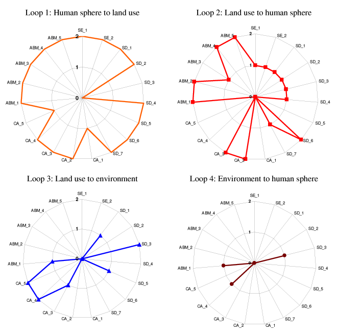
For comparison purposes, we set up an assessment matrix, in which the degree of fulfilment of the four relationships (cf. again Figure 1*) is assigned to each of the models under review. We used a metric scale from 0 to 2: If the criterion is fulfilled, then the “mark” 2 is given; if only parts of the criterion are fulfilled – e.g., the processes implemented by rudimentary or very simple – the “mark” 1 is given; and if the criterion is not at all fulfilled or not included in the model, the “mark” 0 is given. The results of the model assessment are given in forms of simple multicriteria spidergrams which compare the three types of models (SE, SD, CA and ABM; Figure 2*) for all criteria and, in a second range of graphs, all models for each single criterion (Figure 3*).
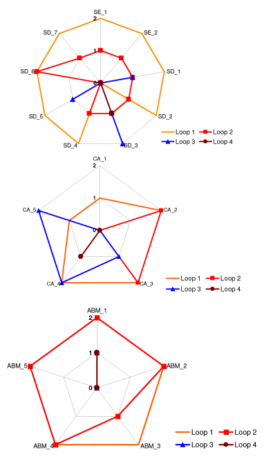
4.2 Relationships between human sphere and land use
Most of the models under review represent the impact of human sphere on land use. Table 1 provides an overview of the model components. Except for three model approaches, each model covers population dynamics and housing or built-up land, which belong to the major variables either for human sphere or land use. The spidergram in Figure 2* clearly shows that causal relationships between human drivers are better captured than the reverse feedback from urban land development to the human drivers. Agent-based approaches mainly cover both loops, since land use variables belong to the neighbourhood of the agents and thus directly influence decision making. In comparison, spatial economics and system dynamics models comprehensively cover loops of type 1 “human sphere to land use,” but mostly neglect effects of changing urban land use on population dynamics or economic development. Cellular automata do include some feedbacks from the effects of land use changes on the human sphere.
4.3 Impact of land use on environment
Only very few simulation models close the loop between driving forces and environmental impacts. Cellular automata perform better in capturing the effects of relatively simple rule-based or neighbourhood-statistic driven land use changes on the environment. Since they are often spatially explicit, landscapes can be more easily represented (cf. again Figure 2*). For example, in CA_3, the impact of urbanisation on biodiversity is assessed, but no feedback to driving forces is taken into account. In SD_7, the impact of transport on the environment is integrated, but it is not clear from the available literature if there is a feedback to driving forces (travel and transportation flows). The two economics models under review (SE_1 and SE_2) lack spatial explicitness to be able to capture a more comprehensive land use relation or feedback.
4.4 Feedback from environment to human sphere
Feedbacks from environmental impacts back to the driving forces that cause urban land use change are mostly realised through changing attractiveness of grid cells or regions for household residential location choices. Those were found in ABM_4 (open space, forest area), ABM_1 (traffic noise, air quality), CA_4 (quality and availability of space for activities), and SD_5 (traffic volume produces air pollution and thus affects human quality of life). In SD_3, the decrease of wetland area (and its negative impact on biodiversity) directly influences decisions to buy land for nature protection instead of further urbanisation. These relationships are the only ones that close the loop from households/individuals as drivers of land use change to environmental impacts and back to the original decision algorithm.
4.5 Feedbacks between local and regional scale
Feedbacks between the local and regional scale can be realised in a variety of ways: first, migration of population within single districts can have an influence on the attractiveness of the districts and therefore influence the housing market in the region, which in turn affects migration. Second, planning and governance on the regional scale can influence local land use changes, which in turn can impact regional planning. In several of the models, the housing market (or price development) is captured implicitly or explicitly. For example, in the spatial economics models SE_1 and SE_2, as well as in the system dynamics models SD_2 and SD_4, the housing market and housing development are explicitly included: In the two former cases in the form of real case study examples (Amsterdam and the U.S.), while in SD_2 an artificial market is created between expansionists and conservationists who want to buy open land – either in order to turn it into urban area or to conserve it. In cellular automata, prices for housing are not explicitly included. Probabilities for land use change can be regarded as bids for (re-)development (CA_2). In some of the agent-based models, real estate markets are already included or are planned to be included (e.g., ABM_1, ABM_3, ABM_5). In these models, developers are agents who can influence the market and therefore also the prices. Governmental planning processes are never explicitly represented in a way that governmental agencies are actors within the model. In some models, planning decisions are integrated as a part of the scenario configuration, e.g., by restricting or promoting possible evolution paths for certain grid cells (e.g., MOLAND). In others, construction and demolition are exogeneous variables (Nijkamp et al., 1993*). But in these cases, planning decisions or housing market trends are not changed during the simulation, so that no feedbacks are established.
 |
 |
 |
Living Rev. Landscape Res., 3 (2009), 2, doi:10.12942/lrlr-2009-2, URL (accessed <date>): http://lrlr.landscapeonline.de/lrlr-2009-2.
 This work is licensed under a Creative Commons License.
© The author(s), except where otherwise noted.
This work is licensed under a Creative Commons License.
© The author(s), except where otherwise noted.